Wheat, Corn, Soybeans and the Major Historical Food Commodity Price Cycles

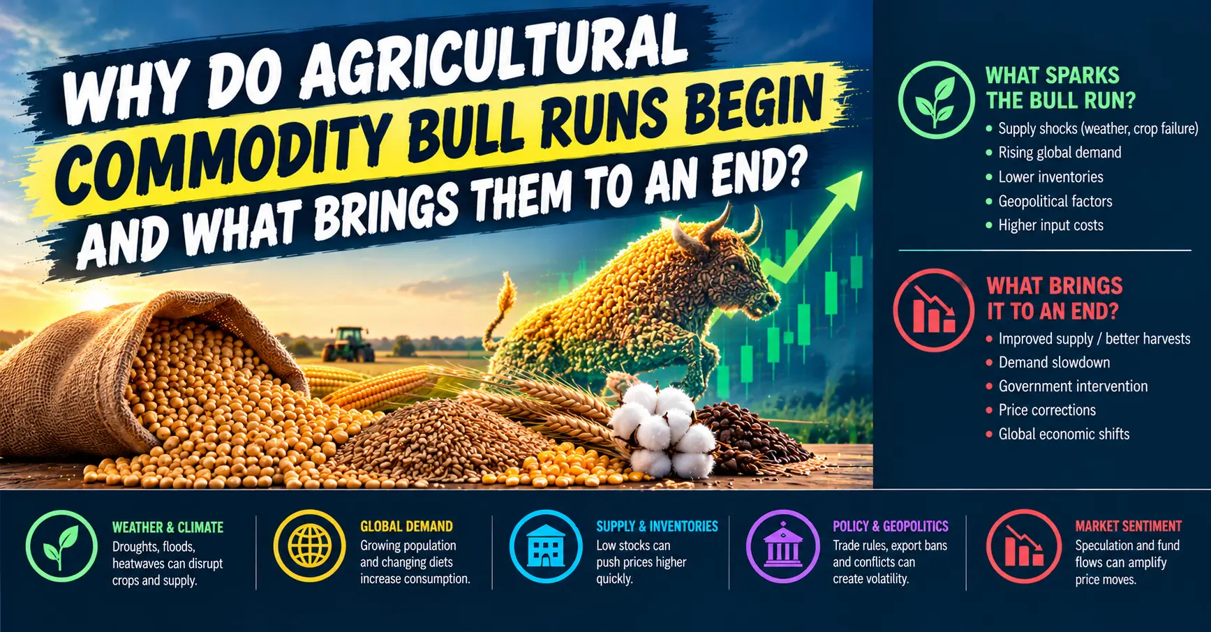
An agricultural commodities bull run occurs because demand rises and supply falls due to poor harvests and inventory shortages. Other factors that can exacerbate price increases include weather risks, export controls, energy prices, biofuel policy, exchange rates, and geopolitics.

The 1971–1974 price rally was caused by growing global demand for grains and poor harvests, while the 1994–1996 rally was characterized by robust Asian demand and short supplies. In the 2006–2008 rally, additional factors were biofuel demand and energy price hikes. Subsequent price spikes were influenced by adverse weather conditions, export controls, economic rebound following the COVID-19 pandemic, and the war between Russia and Ukraine.

This article discusses the drivers and the reversal of these cycles considering wheat, corn, and soybeans, acknowledging that there are separate cycles in sugar, vegetable oils, cocoa, and coffee. In this context, “bull run” is defined as price rises, while “bear phase” is defined as price declines.

1971–1974: Unexpected Grain Demand Meets Poor Harvests

The upsurge in agricultural prices from 1971 to 1974 occurred due to the rise in global grain demand that exceeded the supply. The centrally planned countries, such as the Soviet Union, increased grain imports in the early 1970s. World wheat exports experienced an increase of almost 29% from 1971 to 1972.

Weather conditions also made the situation worse. In 1972, there was a drop in grain production in the United States, Australia, Canada, and the Soviet Union due to poor harvests. There were no reserves that could have helped avoid supply problems. By 1973/74, ending stocks of wheat had dropped considerably compared to 1970/71: 93% in Australia, 64% in Canada, and 59% in the US.

The weakening of the currency and the increase in income levels also played a role in raising prices. In the wake of the dollar’s gold convertibility being suspended in 1971, the US currency weakened and increased the competitiveness of American agricultural products. There was also an increase in income because of increased oil sales.

There was an additional supply problem in the case of soybeans, where Peru suffered from a bad anchovy harvest in 1972, which decreased the supply of fish meal and increased that of soybean meal. Additionally, there were restrictions on exports in some countries, which affected the availability of commodities internationally.

Why the 1971–1974 Bull Run Ended

The rally eventually encouraged a supply response. High crop prices made additional planting and the return of idled land economically attractive. US farmers expanded production, while investment in agricultural infrastructure and export capacity in South America particularly Brazil and Argentina helped establish new sources of grain and oilseed supply. These adjustments could not happen instantly, but they increased the market’s ability to respond over time.

Demand conditions also became less supportive as economic growth and trade momentum softened. As additional production entered the market and consumption no longer grew as quickly as during the initial shock, the supply demand balance improved. Inventories could begin to rebuild, reducing the market’s sensitivity to each new production concern. The key reversal was therefore not one single event: it was the combination of supply expansion, new exporting capacity and a less exceptional demand impulse.

The lesson from this cycle is that an unexpected buyer can ignite a rally when inventories are low, but elevated prices eventually encourage farmers and competing suppliers to bring more product to market.

1994–1996: Strong Asian Demand and Three Years of Weak Grain Production

The 1994–1996 price spike was driven by a combination of stronger demand and disappointing supply. Rapid economic growth in newly industrialised Asian economies supported international trade and increased demand for agricultural products. The expansion of global demand coincided with a decline in grain production for three consecutive years, as major exporting countries experienced below normal harvests.

Inventories amplified the price response. Some countries, including the United States, had reduced carryover stocks and idled cropland to support prices. With smaller reserves available, the market had less capacity to absorb consecutive production shortfalls. The US dollar also depreciated against currencies of major US trading partners during the period, making American agricultural products more competitive in overseas markets and reinforcing export demand.

Why the 1994–1996 Bull Run Ended

The most important demand reversal followed the Asian financial crisis of 1997–1999. The crisis and the resulting slowdown in economic growth weakened demand across affected economies and interrupted the earlier expansion in global trade. As import demand eased, the market no longer faced the same pressure to secure additional grain at increasingly high prices.

At the same time, production incentives and policy changes supported a supply response. The US Federal Agriculture Improvement and Reform Act of 1996 ended the previous acreage reduction programme, making more cropland available for planting. Higher production, weaker demand and improving supply availability shifted the market away from the tight conditions that had driven the rally. A stronger dollar also made US exports relatively more expensive to foreign buyers, adding another headwind.

The defining feature of this reversal was the change in the demand supply balance: the financial crisis weakened demand just as production was able to respond. This cycle shows why monitoring importing country economic growth is important alongside weather and crop inventories.

Source

USDA Economic Research Service: https://www.ers.usda.gov/amber waves/2009/march/agricultural commodity price spikes in the 1970s and 1990s valuable lessons for today   Causes and reversal of the 1994–1996 crop price spike.

2006–Mid 2008: Biofuels, Energy Costs, Poor Harvests and Low Inventories

The 2006–2008 agricultural boom was broader than a conventional weather driven rally. Rising incomes in developing and transition economies increased demand for food, meat, dairy products and vegetable oils. This raised demand for grains and oilseeds used as livestock feed. The value of global agricultural trade increased by more than 50% between 2000 and 2006, reflecting the rapid growth in international demand.

Biofuels introduced an additional structural source of demand. US ethanol production increasingly used corn, while biodiesel production particularly in the European Union added demand for vegetable oils. In the 2007/08 marketing year, ethanol production accounted for about 23% of total US corn use. Corn therefore had to serve food, feed, industrial and fuel markets at the same time. This additional demand altered the relationship between agricultural prices and energy markets.

Higher energy prices also raised the cost of operating farm machinery, transporting crops and producing agricultural inputs such as nitrogen fertiliser. Energy costs could therefore push agricultural prices upward through both production costs and biofuel economics. Meanwhile, production shortfalls caused by adverse weather in 2006–2007 affected major crop producing regions, including wheat production in Australia. The US dollar depreciated, making US exports more competitive, and grain and oilseed inventories became exceptionally tight: the USDA reported aggregate stocks to use ratios below 15%, the lowest level since 1970.

Government policies intensified the imbalance. Some exporters introduced restrictions or taxes to protect domestic consumers, while importers lowered barriers, subsidised consumption or attempted to rebuild stocks. These responses were understandable from a domestic perspective, but export restrictions reduced the quantity available to international buyers. Financial investment may have amplified price moves, but the scale and timing of the rally cannot be attributed to speculation alone; physical supply, demand, stocks, policy and expectations interacted.

Why the 2006–Mid 2008 Bull Run Ended

The global financial crisis changed the outlook for economic growth and commodity demand. As the crisis deepened in 2008, investors and commercial buyers reassessed future consumption, while financial conditions tightened. Agricultural prices fell sharply from their peaks as demand expectations weakened and the acute phase of the market imbalance began to unwind.

High prices also encouraged farmers to expand acreage and production, although crop supply responds with a lag because planting decisions and harvests take time. Biofuel mandates continued to support corn demand, so the price decline did not necessarily imply a return to the much lower price regime of the late 1990s and early 2000s. The reversal was driven by the financial crisis and weaker demand expectations, alongside market adjustment not by biofuel demand disappearing altogether.

The lesson is that a structural demand change can make a rally more powerful, but it does not prevent prices from falling when economic activity contracts or supply adjusts.

 2010–2011: Weather Shocks and Export Restrictions

The 2010–2011 food price spike developed after a sequence of adverse weather events compressed into roughly ten months, beginning in June 2010. Conditions across major producing regions were too dry, too wet, too hot or too cold, sharply reducing expectations for global crop production and stocks. Grain and oilseed consumption continued to rise, so falling production expectations translated quickly into lower projected inventories and higher prices.

A major shock came from the drought and heatwave in Russia and nearby Black Sea regions, which reduced wheat production expectations. Russia imposed a grain export ban in 2010 to protect its domestic market. The restriction reduced internationally available wheat and forced importers to seek alternative supplies. Other weather problems affected corn and oilseed outlooks, including production concerns in the United States and South America. Because several supply risks appeared close together, markets had less time to adjust than during the more spread out 2005–2007 production problems.

The longer term backdrop also mattered. Population and per capita income growth supported demand; consumption of animal products increased; growth in crop yields had slowed compared with earlier decades; energy prices were rising; and biofuel production continued to grow. These structural forces meant that the weather shocks hit markets that were already more sensitive to a supply shortfall.

Why the 2010–2011 Bull Run Eased

The spike eased as crop production and trade adjusted, alternative exporters supplied some of the missing grain, and the immediate panic around availability moderated. High prices encouraged planting and production responses, though the timing differed by crop and region. As new harvest information arrived and supply expectations improved, the market began to price a less extreme shortage.

The 2010–2011 episode should not be treated as if every commodity peaked and declined on the same date. Wheat, corn, soybeans, sugar and vegetable oils had different production calendars, inventory conditions and demand drivers. The common reversal mechanism was a reduction in the expected severity of the shortage, combined with supply responses and changes in demand not one universal event.

2012: US Drought Drives Corn and Soybean Prices Higher

The 2012 rally was more concentrated in grains and oilseeds, particularly corn and soybeans. Severe drought and high temperatures across large parts of the US Midwest damaged crop prospects during critical growing stages. Lower expected yields meant that the market had to reassess how much corn and soybeans would be available for domestic use and exports.

The USDA estimated US corn production at approximately 10.8 billion bushels in 2012, about 13% below 2011. The average yield fell from 147.2 bushels per acre in 2011 to 123.4 bushels per acre in 2012. South American production concerns also affected soybean market expectations. Because futures prices reflect expected future availability, prices could rise as forecasts deteriorated before final harvest figures fully confirmed the damage.

Why the 2012 Rally Eventually Eased

The rally eased as the market began to assess the next crop seasons and the possibility of production recovery. A severe drought can sharply reduce one harvest, but the price response changes when forecasts suggest that subsequent crops may replenish supplies. Farmers can also alter acreage and crop choices in response to relative prices, although planting decisions and weather limit how quickly supply can respond.

The reversal therefore depended on expectations for future yields, planting, demand and inventory rebuilding. It is more accurate to describe this as a drought driven price spike that eventually eased as the outlook changed than to assign the entire reversal to a single event.

2020–2022: Pandemic Recovery Followed by the Russia–Ukraine War

The agricultural price upswing began before the invasion of Ukraine. During the recovery from the initial COVID 19 shock, demand rebounded while pandemic related supply chain constraints, shipping disruptions and logistical bottlenecks remained. Between April 2020 and December 2021, the World Bank’s energy and non energy commodity price indexes rose substantially, reflecting the strong demand recovery and supply constraints across markets.

The invasion of Ukraine in February 2022 intensified the rally. Russia and Ukraine are major exporters of wheat, corn, sunflower oil and other commodities or inputs. The war disrupted production and trade, raised uncertainty about Black Sea shipments and increased the risk premium attached to commodities for which the two countries are important suppliers. The physical disruption of ports and productive capacity, sanctions and changes in trade patterns all affected the market.

Higher energy prices raised the cost of producing and transporting agricultural goods, while natural gas an important input in nitrogen fertiliser production pushed fertiliser costs higher. These input cost pressures created a risk that farmers would reduce fertiliser use or alter planting decisions, potentially affecting future output. Export restrictions and other protective policies further reduced the flexibility of global trade. Wheat and edible oils were particularly exposed to the Russia–Ukraine shock, while corn and soybeans were affected through feed markets, substitution and broader supply demand conditions.

Why the 2020–2022 Bull Run Reversed from Its Peak

Prices began easing from their 2022 peaks as the most acute market disruption moderated. The resumption of some Ukrainian grain exports through the Black Sea improved availability. Better than expected harvests and larger supplies of some oilseeds also eased pressure. At the same time, concerns about weaker global growth and recession reduced expectations for future demand.

The World Bank noted in October 2022 that many commodity prices had declined from their recent peaks amid weaker growth prospects. It also attributed the expected easing in agricultural prices to a better than projected global wheat crop, stable rice supplies and the resumption of Ukrainian grain exports. The decline was not a return to a risk free market: continued war, sanctions, energy price volatility and trade restrictions remained potential sources of renewed price pressure.

The key lesson is that a geopolitical shock can accelerate a rally when inventories are already tight, but prices can retreat when trade routes reopen, alternative supply becomes available, harvest expectations improve or demand expectations weaken.

What Repeatedly Starts an Agricultural Bull Run?

The first common factor is a tightening balance between demand and available supply. Demand may grow because of population growth, rising incomes, changing diets, livestock feed needs or new industrial uses such as biofuels. The price impact is much greater when production fails to keep pace. A large unexpected buyer, as in the early 1970s, or a structural new source of demand, as with corn ethanol in the 2000s, can shift the market balance quickly.

The second common factor is a supply shock. Drought, heat, excessive rain, crop disease, low yields, war or damaged transport infrastructure can reduce expected production or prevent crops from reaching buyers. Markets usually react to expected harvests, not just final production numbers, so prices can move before the shortfall is confirmed.

The third common factor is the macroeconomic and input cost environment. A weaker US dollar can support dollar denominated agricultural prices by making exports more competitive. Higher energy prices can raise fertiliser, fuel and freight costs, while also improving the economics of biofuel production. These channels are especially relevant when they occur at the same time as low inventories and weather related production problems.

Finally, demand substitution and crop specific linkages matter. Soybean meal can benefit when other protein feed sources become scarce; corn can be affected by ethanol demand; vegetable oils can respond to biodiesel demand; and sugar can move with the sugar versus ethanol allocation decision. A bull market can therefore be broad based or concentrated in one commodity, depending on the shock.

What Repeatedly Ends an Agricultural Bull Run?

The most persistent bear market driver is a supply response. High prices encourage farmers to plant more, expand acreage, invest in inputs or improve yields. Competing producing countries may also expand export capacity. Because crops have growing seasons and biological limits, the response is delayed; once new supply arrives, however, the market can move from scarcity toward surplus.

The second common factor is demand destruction or normalisation. Very high prices can reduce consumption, encourage substitution and weaken demand from importers. Economic slowdowns and financial crises can also reduce purchasing power, as happened after the 1994–1996 rally and during the 2008 financial crisis. A bull run can end even without a dramatic recovery in production if demand weakens enough to close the gap.

A final qualification is essential: agricultural commodities do not all enter a bear market together. The correct question is not simply whether agriculture is bullish or bearish, but which crop is tight, where the shortage is located, and whether the next supply response is sufficient.

 Why Are We Focusing on These Four Crops?

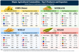
  Corn, soybeans, wheat and sugar have been selected because of their importance in global food supply, agricultural trade and commodity price cycles. These crops have historically experienced significant price rallies when adverse weather, falling inventories, rising demand, export restrictions or geopolitical disruptions constrain supply.

  Rather than analysing hundreds of agricultural commodities, focusing on these four allows us to study the major drivers of agricultural bull runs and understand how supply demand imbalances translate into price increases. They also represent different parts of the agricultural value chain, from staple food grains and animal feed to vegetable oils, biofuels and sugar.

Source – Security Exchange Commision

Why Are We Focusing on Major Producing and Exporting Countries?

  The next step is to narrow our analysis to the countries that dominate production and international trade for each crop. For example, the United States, Brazil and Argentina are major players in corn and soybean markets, while the European Union, China, India and Russia are important in wheat, and Brazil, India and Thailand are key sugar producers.

Tracking these countries helps us identify where production risks emerge, how weather affects harvests, which countries control export availability and how disruptions can influence global prices. This approach takes us from historical bull run drivers, to four key crops, and finally to the countries and value chains most capable of influencing their global supply and prices.

CORN

Brazil’s corn production: Is it following the same trend?

Brazil’s corn sector has also expanded substantially, although the latest crop estimates are less straightforward than those for soybeans.

Conab’s latest 2025/26 estimates reported by World Grain put total corn production at approximately 141.7 million tonnes. The forecast includes three corn crops, with the second crop, known as safrinha, accounting for the majority of output. (World Grain)

Crop year	Corn production	Status
2024/25	Approximately 142.3 million tonnes	Previous crop
2025/26	Approximately 141.7 million tonnes	Slightly lower than the previous crop
2026/27	Initial USDA forecast indicates growth of approximately 6.2% against its initial forecast for 2025/26	Forecast; not final production

The 2024/25 figure is calculated from the reported 2025/26 estimate of 141.72 million tonnes and the reported 0.4% year on year decline. The 6.2% figure for 2026/27 refers to the change between initial USDA forecasts, not necessarily the final year on year production change.

 

Why does the second corn crop matter?

   Brazil commonly plants corn after harvesting soybeans. This allows farmers to grow two crops on the same land during a growing cycle.

However, it also creates a link between soybean and corn production:

1. Soybeans are planted and harvested.
2. Farmers plant the second corn crop.
3. Delayed soybean planting or harvesting can push corn planting later.
4. Later planting can expose corn to less favourable rainfall and increase yield risk.

Regional Impacts on Corn and Agriculture in Brazil

1. Central-West (Mato Grosso, Goiás and Mato Grosso do Sul):

Brazil’s main corn- and soybean-producing region is facing irregular rainfall, prolonged dry spells and extreme heat. In Mato Grosso, the agricultural economics institute Imea expects lower yields for the 2026–27 second-crop corn harvest due to drier conditions and potential delays in soybean planting. Since safrinha corn is planted after soybeans are harvested, delays can push planting beyond the optimal window, exposing the crop to greater weather-related risks.

2. North and Northeast:

These regions face the risk of severe drought and below-normal rainfall, which could hamper soil moisture and early crop establishment. If dry conditions persist during critical growth stages, crop development and yields could come under pressure.

3. South (Rio Grande do Sul, Paraná and Santa Catarina):
In contrast to the dry conditions threatening central and northern Brazil, the southern states face the risk of excessive rainfall, severe storms and flooding associated with El Niño. Heavy precipitation could disrupt planting and other field operations, waterlog soils and potentially damage crops.

The main problems facing Brazilian farmers

1. Fertiliser costs and import dependence

Brazil depends heavily on imported fertilisers. Purdue reports that imports accounted for approximately 88% of fertiliser consumption in 2025.

Higher fertiliser costs create a particular problem because farmers need to finance inputs before harvesting and receiving revenue from their crops. If input prices rise while soybean prices remain weak, margins become tighter.

Farmers may respond by reducing fertiliser application or other expenditure. This may not prevent planting, but it could reduce yields and make production forecasts harder to achieve.

2. Expensive credit and weak profitability

High interest rates make it more expensive to finance seeds, fertilisers, machinery and other farming expenses.

Purdue’s June 2026 analysis notes that Brazilian farmers are facing tighter credit conditions, rising debt and weaker profit margins. These pressures could slow investment or acreage expansion.

Nevertheless, the historical record suggests that economic pressure alone has not consistently stopped Brazilian production from growing.

3. El Niño and weather uncertainty

Weather is potentially the most important short term production risk.

    Purdue warns that El Niño related conditions could affect rainfall distribution across Brazil during the 2026/27 crop season. Some regions may face reduced rainfall, while others could experience excessive rain.

   Brazil’s North and Central West regions are facing the risk of below average rainfall and excessive heat associated with the developing El Niño, threatening soybean and corn production. The Central West, particularly Mato Grosso, is a major producer of both crops.

Drought could reduce soybean yields and delay harvesting, subsequently narrowing the planting window for second crop corn (safrinha), which is planted after soybeans. If these weather conditions persist, Brazil’s expected record soybean production and corn output could fall short of forecasts, potentially supporting global commodity prices. However, actual crop losses are not yet confirmed and will depend on rainfall patterns and crop conditions.

 United States: Corn Production, Weather Risks and Rising Production Costs

The United States is heading towards another exceptionally large corn harvest in the 2026/27 marketing year. According to the USDA, in September 2026, US corn yield was estimated at 178.5 bushels/acre, with production of 15.8 billion bushels & US corn inventories stood at 1.551 billion bushels in September 2025, rising to 2.095 billion bushels in September 2026, up 35% YoY & in October 9, 2026, report, corn production is forecast at approximately 16.03 billion bushels, with an average yield of 181.2 bushels per acre & projected ending stocks increased to 1.849 billion bushels.

Despite adverse weather in some growing regions, higher estimated yields have lifted the production forecast. However, the combination of delayed harvesting, weakening crop conditions and rising input costs is creating additional pressure on farmers’ profitability.

Production, Acreage and Inventories

US corn planted acreage is estimated at 95.3 million acres, down approximately 3% from 2025, while the area expected to be harvested for grain has declined by around 4% to 87.4 million acres. Higher expected yields are offsetting the reduction in acreage. Meanwhile, corn stocks on September 1, 2026, reached approximately 2.10 billion bushels, up 35% year on year, indicating that the US entered the new marketing year with substantially more old crop corn in storage. The combination of higher production and larger inventories points towards a well supplied market, potentially limiting price increases unless demand strengthens or production estimates decline.

Weather Conditions: Heat, Dryness and Harvest Delays

Weather conditions have been uneven across the Corn Belt. Earlier heat and dry conditions raised concerns about crop development in some regions, while excessive rainfall in parts of the Midwest subsequently delayed harvesting. As of October 4, 23% of the US corn crop had been harvested, compared with the five year average of 27%. Furthermore, the share of corn rated good or excellent fell to 54%, its lowest level of the season. In Iowa, a historically wet September left some fields too saturated for machinery, although a subsequent period of warmer, drier weather improved field conditions. These delays can increase drying costs, disrupt grain deliveries and raise the risk of quality deterioration. However, slower harvesting does not automatically imply lower production, and the USDA’s latest forecast still indicates a large crop.

Diesel Crisis: Rising Harvesting and Transportation Costs

US farmers are also facing a significant increase in diesel prices, driven by disruptions to global fuel supplies associated with the conflict involving Iran and attacks on Russian refineries. According to Reuters, the average US retail diesel price reached $6.29 per gallon in September 2026, approximately 68% higher than a year earlier. Diesel is essential for tractors, combines, grain drying equipment and trucks transporting corn from farms to storage facilities and processing plants. Reuters reported that one South Dakota farmer expected to spend as much as $1,500 per day on fuel for a single combine, approximately double the previous year’s cost. These higher expenses are squeezing margins during the critical harvesting period, when farmers cannot simply postpone essential operations because fuel has become more expensive.

Fertiliser, Input Costs and Farm Profitability

Higher energy prices are also increasing the cost of fertilisers and other agricultural inputs. Nitrogen fertiliser production is energy intensive, making prices vulnerable to disruptions in natural gas and other energy markets. The University of Arkansas estimated that higher diesel and urea costs together could add approximately $97.73 per acre to corn production costs in Arkansas in 2026, based on its assumptions and price data. Separately, USDA forecasts that total US farm production expenses will reach $492.8 billion in 2026, up 4.5% from 2025. These figures show that farmers are facing pressure from multiple directions: fuel, fertiliser, transportation and financing costs are rising, while abundant corn supplies can limit their ability to pass those expenses on through higher selling prices.

Demand and the Outlook for Prices

US corn demand continues to receive support from ethanol production, livestock feed and exports. However, the USDA’s October outlook indicates that supplies are increasing substantially, with 2026/27 US feed grain supply forecast at 476.4 million tonnes, the second highest level on record. This creates a difficult situation for farmers: production remains strong, but the cost of producing and delivering each bushel has increased sharply. Rising input costs may eventually influence planting decisions for the next crop season, potentially affecting acreage or fertiliser application. Nevertheless, higher production costs do not automatically translate into higher corn futures prices; prices will depend primarily on the balance between supply, demand and inventories.

 Key Takeaway – USA & Brazil Corn

The US and Brazil are facing a dual pressure from rising diesel and fertilizer costs, which could squeeze corn farmers’ margins and influence future production decisions. In the US, diesel prices surged during 2026, while higher urea and nitrogen fertilizer costs added to production expenses. A University of Arkansas analysis estimated that diesel and urea price increases together could add $97.73 per acre to corn production costs in the state.

Brazil faces an additional vulnerability because it imported around 88% of its fertilizer requirements in 2025. Higher global fertilizer prices, expensive credit and tight farm margins could discourage acreage expansion or reduce input use for the 2026–27 crop. Although the US currently has a strong corn production outlook, these rising costs in both countries could weigh on future supply growth. However, higher costs do not automatically mean lower production the eventual impact will depend on farmers’ input decisions, weather conditions and actual yields

 SOYABEAN

BRAZIL

Brazil’s agricultural sector has continued expanding despite higher fertiliser costs, expensive credit and pressure on farmers’ profit margins. The latest reports from Reuters, World Grain, OFI Magazine and Purdue University show an important trend: Brazil’s soybean production is reaching consecutive records, while its planted area continues to expand. However, production growth in 2026/27 faces greater economic and weather related risks.

1. Brazil’s soybean production: Last two years and 2026/27 forecast

According to Conab estimates reported by World Grain and OFI Magazine, Brazil’s soybean production reached approximately 172.5 million tonnes in 2024/25 and is estimated at 180.4 million tonnes in 2025/26. The USDA’s forecast for 2026/27 is higher still, at 184 million tonnes.

Crop year	Soybean production	Year on year change	Status
2024/25	172.5 million tonnes		Record harvest
2025/26	180.4 million tonnes	+4.6%	New record
2026/27	184 million tonnes	+2.0%	USDA forecast

What does this tell us?

• Production increased by approximately 7.9 million tonnes between 2024/25 and 2025/26.
• The next crop is forecast to add another 3.6 million tonnes.
• If the 2026/27 forecast is realised, Brazil will achieve its third consecutive record soybean harvest.

The main driver is the expansion of planted area, supported by improved cultivation practices and investment in agricultural technology. However, higher production costs and weather risks could prevent the next crop from reaching its projected level.

Reuters’ March 2025 article discussed the possibility of another record Brazilian soybean crop in 2025/26. At the time, early estimates suggested production of 173 million tonnes, approximately 2% above the previous year’s level.

Reuters also highlighted a historical forecasting issue: the USDA and Conab had frequently underestimated Brazilian production, partly because they underestimated planted area.

The eventual estimates subsequently increased. This illustrates why early season production forecasts should not be treated as final numbers.

2. Soybean acreage: How much land is Brazil planting?

Acreage expansion is the most important long term driver of Brazil’s soybean production growth.

   According to OFI Magazine’s report on the USDA forecast, soybean planted area is expected to increase from approximately 49 million hectares in 2025/26 to 50.5 million hectares in 2026/27. (Oils & Fats International)

Crop year	Soybean planted area	Annual change
2024/25	Approximately 47.7 million hectares
2025/26	Approximately 49.0 million hectares	+2.7%
2026/27	50.5 million hectares	Approximately +3.1%

 

Why is acreage increasing?

1. More land is being allocated to soybeans.

Brazilian farmers have consistently expanded soybean cultivation over the past two decades. Purdue University’s June 2026 analysis notes that soybean area has more than doubled since 2011.

2. New agricultural regions are contributing to growth.

The USDA forecast identifies the MATOPIBA region, covering parts of Maranhão, Tocantins, Piauí and Bahia, as an important area for further expansion.

3. Infrastructure investment can make new land more commercially attractive.

Roads, waterways, storage and export infrastructure can improve the economics of cultivation in developing agricultural regions.

But there is an important warning

Although acreage is still expected to expand, the growth rate may slow.

The USDA forecast reported by OFI Magazine identifies economic uncertainty and potential climate problems as constraints on future expansion. A separate Reuters report also highlighted rising production costs and the risk of weaker farmer profitability.

 USA

USA Soybean Production: September vs October 2026

In September 2026, the USDA estimated US soybean yield at 52.8 bushels per acre, an increase of 0.1 bushel per acre from the August estimate. Production was projected at approximately 4.5 billion bushels, with the estimate slightly increasing from the previous month.

In October 2026, the USDA raised its soybean yield estimate to 53.1 bushels per acre and projected total production at approximately 4.562 billion bushels, a record crop. Compared with September’s estimate of approximately 4.535 billion bushels, the October projection represented an increase of around 27 million bushels. The season average soybean price forecast remained unchanged at $12 per bushel. The higher production estimate suggests improved supply availability, although the final market impact will also depend on export demand, domestic crushing and soybean product demand.

US soybean inventories, however, followed a different trend from corn. USDA data show that soybean stocks were 325 million bushels on September 1, 2025, compared with 315 million bushels on September 1, 2026, a decline of approximately 3% year on year. This means that, despite the larger expected new crop, US soybean inventories at the beginning of the 2026/27 marketing year were slightly lower than a year earlier. Soybean stocks on June 1, 2026, stood at approximately 1.061 billion bushels.

USA Soybean: Weather in Major Growing States (October 2026)

Iowa, Illinois, Minnesota and Indiana are among the major US soybean producing states. In late September and early October, heavy rainfall across parts of the Midwest disrupted fieldwork, particularly in Iowa. However, drier weather subsequently helped harvesting resume. As of October 11, 46% of the US soybean crop had been harvested, 4 percentage points below the five year average.

 SUGAR

1. BRAZIL World’s Largest Sugar Producer and Exporter

Adding to supply concerns, S&P Global Energy CERA revised its global sugar balance for the 2025 26 season from a surplus of 1.36 million tonnes to a deficit of 540,000 tonnes. The revision followed a reduction in Brazil’s Center South cane crushing estimates for September due to above average rainfall.

Production & Global Share: Brazil accounts for approximately 24% of global sugar production and around 46% of global sugar exports, making it the most influential country in determining internationally traded sugar supply. According to CONAB’s 2026/27 estimates, sugarcane production is projected at 705.2 MMT, up 4.7% YoY. However, sugar production is estimated at 42.89 MMT, down 2.9% YoY, despite higher cane availability.

Weather & Crop Conditions: Brazil’s key sugar producing region is the Centre South, particularly São Paulo, which accounts for approximately 90% of national sugar and cane production. Excess rainfall around São Paulo and the Centre South delayed harvesting and crushing, while excessive moisture can dilute sugar concentration and reduce recoverable sugar (ATR). Conversely, periods of heat and low rainfall in São Paulo, Goiás and Minas Gerais create risks to cane development and recovery. CONAB’s latest assessment nevertheless indicates improved national productivity of 77.9 tonnes/hectare, up 3.6%, supported by favourable climatic conditions earlier in the crop cycle.

Key Supply Driver   Sugar vs Ethanol: The critical factor is how much sugarcane mills allocate to sugar production versus ethanol. Cane based ethanol production is forecast at 29.98 billion litres, up 9.7% YoY, while sugar production is expected to decline. Brazil’s ethanol blend mandate also increased from 30% to 32% in August 2026. Mills have directed 53.8 per cent of available cane sugar content (ATR) to ethanol so far this season, compared with 47.7 per cent a year earlier. If more cane is diverted towards ethanol, less sugar may be available for export, potentially supporting international prices. Brazil’s raw sugar exports in August were 2.7 million tonnes, down from 3.7 million tonnes a year earlier. Exports from January to August were 2.2 million tonnes lower year on year, the report said.

The key monitorables are weather, sugar recovery (ATR), the sugar ethanol mix and export volumes.

2. INDIA 🇮🇳   World’s Second Largest Sugar Producer

Production & Global Share: India accounts for approximately 16% of global sugar production. The blog estimates that Indian sugar production for 2025/26 has been revised down to approximately 280LMT (28MMT), from an initial estimate of 343 LMT. The shortfall has been attributed to excessive rainfall, waterlogging and crop diseases. India’s annual domestic sugar consumption is approximately 280–290 LMT, making domestic production and inventory levels critical to the country’s sugar balance.

Weather & Crop Conditions: India’s sugar production is concentrated in three states: Maharashtra, Uttar Pradesh and Karnataka. As of 30 April 2026, Maharashtra produced 99.20 LMT, Uttar Pradesh 89.65 LMT, and Karnataka 48.01 LMT. Excess rainfall and waterlogging have affected crop conditions, while Red Rot and Top Borer have reduced cane yield and quality in affected areas. Karnataka is also facing concerns over inadequate rainfall and disease, although the reported potential production decline of around 30% is an industry association estimate, not an official government forecast.

Maharashtra, India’s largest sugar producing state, is facing a weaker sugarcane outlook for the 2026–27 season due to below normal rainfall, higher temperatures and declining soil moisture. According to ChiniMandi, the state’s sugar production estimate was revised down to 90.18 lakh tonnes, from an earlier estimate of 102.5 lakh tonnes. Sugarcane production is projected at 1,127 lakh tonnes, compared with 1,316 lakh tonnes in 2025–26.

ChiniMandi reported that Maharashtra declared drought in 265 of its 358 talukas in September 2026, following an 18.8% rainfall deficit. Lower reservoir levels could restrict irrigation and create water shortages during January and February, potentially affecting late season crushing. The Western India Sugar Mills Association has estimated that sugar production could decline by around 20% to approximately 80 lakh tonnes, although this is an industry estimate rather than an official forecast.

UP produced 89.65 LMT, accounting for 32.6% of the reported state wise production. The state’s key concerns include declining cane acreage, rising cultivation costs and Red Rot disease, which has affected the widely cultivated CO 0238 variety. These factors could constrain cane availability and affect sugar recovery.\

Karnataka: Karnataka produced 48.01 LMT, accounting for 17.4% of reported production. The key risks are inadequate rainfall, disease and declining cane availability. The Karnataka State Sugarcane Growers’ Association has warned that cane production could fall by around 30%

Key Takeaway: India’s sugar outlook is increasingly dependent on weather conditions, disease incidence and sugar recovery in its three major producing states. Maharashtra faces the risk of lower cane availability due to deficient rainfall and declining soil moisture, while Uttar Pradesh faces disease related risks and declining acreage. Karnataka’s concerns centre on inadequate rainfall and disease related crop losses. If these conditions reduce sugar production while domestic consumption remains around 280–290 LMT annually, India’s sugar balance could tighten further.

 THAILAND World’s Third Largest Sugar Exporter

Production & Global Share: Thailand accounts for approximately 8% of global sugar exports. According to the USDA’s April 2026 report, sugar production for 2026/27 is forecast at 9.5 MMT, down 16% YoY, while exports are projected to decline by 14% to 6 MMT. Lower sugarcane availability and reduced planted area are expected to constrain exportable supply.

Weather & Crop Conditions: Thailand faces growing drought risks as a strong El Niño develops. Rainfall in the northeastern region which accounts for approximately 45% of national sugarcane production has been below normal. Sugarcane production could fall to around 100 MMT in 2026/27 from 106 MMT in the previous season, according to industry estimates. Higher temperatures, water shortages and the possibility of farmers shifting to cassava could further affect cane yields.

Inventory & Global Price Impact: USDA estimates place Thailand’s ending sugar stocks at approximately 12.45 MMT for 2026/27, up from 12.25 MMT in 2025/26. Despite lower production, these substantial projected inventories could cushion the impact on export availability. Meanwhile, ChiniMandi, citing S&P Global, reported on October 16 that Thai raw sugar prices had reached a 22 month high, amid Brazilian crushing disruptions and a revision in the global sugar balance from a 1.36 MMT surplus to a 0.54 MMT deficit. However, subdued physical demand raises questions about the rally’s sustainability.

 WHEAT

Canada Wheat: El Niño Threat, Climate Risks and Harvest Disruptions

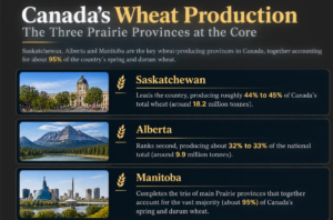
Canada is one of the world’s major wheat producers and exporters, and its wheat supply is heavily concentrated in three Prairie provinces: Saskatchewan, Alberta and Manitoba. Together, these provinces account for approximately 95% of Canada’s spring and durum wheat production, making their weather conditions particularly important for global wheat supply.

1. Three Provinces, One Critical Wheat Belt

Saskatchewan is Canada’s leading wheat-producing province, contributing approximately 45% of national wheat production. Alberta ranks second, accounting for roughly one-third, while Manitoba completes the Prairie region’s dominant production base. Their combined importance means that drought, excessive rainfall or extreme temperatures across these provinces can have significant consequences for Canada’s wheat harvest.

Statistics Canada’s September 2026 estimates projected Canadian wheat production at 36.1 million tonnes, down 10.9% year-on-year. Production was expected to decline to 16.9 million tonnes in Saskatchewan, 10.9 million tonnes in Alberta and 4.9 million tonnes in Manitoba. These estimates were already pointing to a smaller crop before the full impact of subsequent harvest delays was assessed.

2. Climate Change and the Developing El Niño

Canada’s Prairie wheat belt faces a growing challenge from increasingly variable weather conditions. The Canadian Climate Change Report 2026 projects that summer droughts could become longer, more intense and more frequent across central and southern Canada as global warming increases. This raises concerns about soil moisture, crop development and water availability during critical growing periods.

A developing El Niño adds another variable to the 2026–27 agricultural outlook. The drought outlook discussed in the supplied video highlights the possibility of warmer and drier conditions in parts of Western Canada, particularly where soil moisture is already low. Saskatchewan and Manitoba face risks if limited winter precipitation is followed by weak spring rainfall and persistent summer dryness. In Alberta, water availability in southern river basins and irrigation-dependent areas will also be important.

However, El Niño does not automatically mean a severe drought across all three provinces. The video describes an emerging El Niño pattern and potential regional risks; it does not establish that a severe El Niño or a nationwide agricultural drought is certain. Winter snowpack, spring precipitation and summer temperatures will determine how much water is available to crops.

3. The Immediate Warning: Excessive Rainfall Has Already Damaged Harvest Quality

While the next growing season faces potential drought risks, Canada’s 2026 harvest has already experienced the opposite problem: excessive rainfall and waterlogged fields.

According to Reuters’ September 15 report, persistent rain delayed harvesting across Saskatchewan, Alberta and Manitoba. By September 7, Saskatchewan had harvested just 27% of its crop, compared with a five-year average of 58%. Alberta’s harvest was approximately 21% complete by September 8, against its five-year average of 43.5%.

The problem extends beyond delayed harvesting. Prolonged exposure to moisture can cause wheat kernels to sprout, lose colour and weight, or develop mould and fungal damage. These problems can downgrade wheat from premium food-quality grades to lower grades, reducing farmers’ selling prices and the availability of high-quality grain for millers.

This distinction matters for global markets: Canada could face pressure on exportable milling-quality wheat even if the eventual reduction in total production is less severe than feared. Official estimates reflecting the full damage from late-season rain were not yet available in the September report.

4. What This Means for Global Wheat Supply

Canada’s wheat outlook presents two different weather risks across consecutive agricultural periods:

• 2026 harvest: Excess rainfall and delayed harvesting threaten grain quality, potentially reducing the supply of premium milling wheat.
• 2027 growing season: Developing El Niño conditions could increase the risk of heat and moisture stress in vulnerable regions if winter snowpack and spring rainfall prove insufficient.

Because Saskatchewan, Alberta and Manitoba dominate Canada’s spring and durum wheat production, adverse conditions across these provinces could affect the country’s exportable supply. However, the extent of any impact on global wheat prices will depend on actual production losses, grain quality, export availability and competing exporters’ harvests.

Australia Wheat: El Niño & Export Supply Risks

Australia is one of the world’s leading wheat exporters, with domestic consumption of approximately 6.5–7 million tonnes against annual production of around 30–36 million tonnes. Consequently, changes in Australian production can significantly influence global wheat availability.

1. Production Outlook: 2026–27

Australia’s wheat production is forecast to decline by approximately 17% year-on-year to 29.9 million tonnes, compared with around 36 million tonnes in the previous season. The decline reflects reduced planted area and weaker yield expectations in some regions. However, production is still expected to remain above its ten-year average. Miller Magazine

2. Climate Change & El Niño Risk

A developing strong El Niño raises concerns about warmer temperatures and below-average rainfall, particularly across eastern Australia. Insufficient moisture during critical crop-development stages could further reduce wheat yields. However, improved rainfall in parts of southern and western Australia may offset some regional losses. The Australian Bureau of Meteorology’s El Niño monitoring data remains an important indicator to watch. Australian Bureau of Meteorology

3. Export Impact & Key Takeaway

Australia’s wheat exports are forecast at approximately 24.5 million tonnes for 2026–27. Existing stocks could cushion the impact of lower production, but further weather-related losses may tighten export availability for international buyers. World-Grain.com

Key takeaway: Australia’s wheat crop faces a potential downside risk from El Niño, particularly if eastern growing regions experience prolonged dryness and heat. However, a nationwide crop failure is not the baseline forecast. Monitor spring rainfall, final yields and export availability to assess the impact on global wheat prices.

 USA Wheat: Severe Drought & Tight Export Supply

The United States is facing a major wheat production setback in the 2026–27 season, primarily due to severe drought across the Great Plains. USA Production vs. Domestic Consumption

• Production (2026–27 forecast): 1.534 billion bushels (~41.7 million metric tonnes) as per High Plain Journal .This represents an approximately 22.7% decline from the previous year’s production of 1.985 billion bushels.
• Production (2025–26): 1.985 billion bushels (~54.0 million metric tonnes).
• Domestic Consumption (2026–27 forecast): 1.099 billion bushels (~29.9 million metric tonnes).

What Does This Mean?

US wheat production is forecast to fall significantly, while domestic consumption remains substantial. Based on these figures, production would exceed domestic consumption by approximately 435 million bushels.

However, this difference is not the same as exportable surplus. The US must also account for beginning stocks, imports, exports and ending inventories. The USDA’s October 2026 outlook separately forecasts US wheat exports at 750 million bushels, highlighting the pressure on export availability.

 The biggest concern is Hard Red Winter (HRW) wheat, a major variety used in bread production, grown mainly across states such as Kansas, Oklahoma and Texas. Prolonged dryness reduced soil moisture and damaged crop yields, while the long-term decline in US wheat acreage has further constrained production.

1. Climate Change & El Niño Risk

Drought has been a major factor behind the smaller crop. Although rainfall has improved conditions in some areas, late-season rain cannot fully reverse damage already suffered by the harvested winter wheat crop. Meanwhile, developing El Niño conditions could influence temperatures and rainfall patterns during the upcoming growing season. However, its precise impact on US wheat production remains uncertain; the key indicators to watch are soil moisture, winter wheat planting progress and rainfall across the Great Plains.

2. Export Impact & Global Supply

The production shortfall is affecting the US export outlook. In its October 2026 outlook, the USDA reduced projected US wheat exports for 2026–27 by 25 million bushels to 750 million bushels the second-lowest level since 1971–72. Hard Red Winter wheat exports are forecast at just 175 million bushels, the second-lowest on record, reflecting tight supplies and weaker export sales. US wheat ending stocks are projected at 740 million bushels, around 20% below the previous year, even after the latest upward revision.

This matters because lower US export availability can reduce the supply accessible to international buyers. However, the global price impact will also depend on production and exports from major competitors such as Russia, Canada and Australia. If these suppliers experience weather-related losses at the same time, global wheat markets could face additional pressure.

Do Falling Bond Yields Signal the Beginning of a Commodity Bull Market?

1. The Historical Evidence: Three Important Instances

Case 1: 2000–2008 — The Commodity Supercycle

This is one of the most relevant periods to investigate for your hypothesis.

What happened?

• 2000–2002: The dot-com bubble burst, and US equity markets experienced a major decline.
• 2000–2003: US Treasury yields generally declined from their earlier highs.
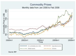
• 2002–2008: A major commodity bull market developed, with prices rising across energy, metals and several agricultural commodities.

Research published in the World Development journal identifies a major commodity supercycle beginning around 2000. The boom was closely associated with global economic expansion, particularly strong demand from emerging economies. (ScienceDirect)

The Bank of Canada also identifies the 2006–2008 commodity boom as being driven substantially by increased demand, much of it originating in Asia. Financial leverage and elevated asset prices also contributed. (Bank of Canada)

 Case 2: 2008–2011 — Financial Crisis Followed by a Commodity Recovery

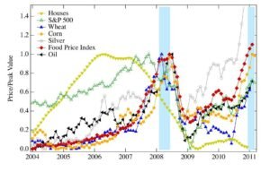
This period is particularly useful because it shows both the potential relationship and its limitations.

What happened?

Phase 1: 2008 financial crisis

• Equity markets crashed.
• Investors sought safety in government bonds, while central banks cut interest rates.
• Commodity prices also collapsed as global demand expectations deteriorated.

Phase 2: 2009–2011 recovery

• Global economic activity began recovering.
• Monetary policy remained highly accommodative.
• Demand for industrial commodities recovered, while supply constraints and geopolitical developments affected individual markets.
• Many commodity prices rose substantially from their crisis lows.

The Bank of Canada discusses the earlier commodity boom and the subsequent global financial crisis as distinct phases, highlighting the importance of economic demand and financial conditions. (Bank of Canada)

 Case 3: 2020–2022 — Falling Yields, Then a Powerful Commodity Rally

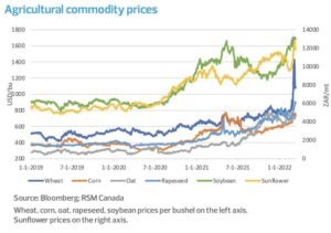
This period is particularly relevant to your research into agricultural commodities.

What happened?

2020:

• The pandemic triggered a sharp market sell-off.
• Treasury yields fell as investors sought safety and central banks eased monetary policy.
• Commodity markets initially experienced severe disruptions, with demand collapsing in some sectors.

2021–2022:

• Economic reopening increased demand for energy, industrial inputs and agricultural products.
• Supply chains struggled to keep pace with recovering demand.
• Russia’s invasion of Ukraine in February 2022 intensified disruptions to energy, grain and fertiliser markets.
• Many commodity prices surged.

The IMF’s research on commodity price cycles documents how commodity booms can reflect a combination of global demand, supply constraints and changing macroeconomic conditions. (IMF eLibrary)

2. The Important Distinction: Why Are Bond Yields Falling?

Bhai, this is the most important part of your hypothesis.

Falling yields can signal two very different economic situations.

Scenario	Why yields fall	Potential impact on commodities
Scenario A: Economic slowdown	Investors expect weaker growth and seek safety in government bonds.	Commodity demand may weaken, putting downward pressure on prices.
Scenario B: Supply shock	Yields fall because growth expectations deteriorate, while a supply disruption reduces commodity availability.	Commodities can rise even as equities weaken and yields fall.

3. My Conclusion for Your Commodity Bull-Run Article

Examples from history show that falling yields may happen at the same time as the beginning of a commodity bull run, although the latter does not necessarily follow as a result of that. The 2000-2008 supercycle came after the dot-com bust, whereas the 2020-2022 bull run took place following the pandemic-induced monetary loosening. The financial crisis of 2008 proved that falling yields and commodities went hand-in-hand even as stocks fell.

 Conclusion

Positive prospects for crops in the US and Brazil should aid supply, although drought, decreasing wheat production, and disruption in exports elsewhere may result in tighter supplies. High diesel prices, fertilizer, shipping, and borrowing costs are putting pressure on farmers’ margins, possibly constraining future production, although reduced production is not assured.

Decreasing bond yields have been linked to an increase in commodity prices, as in the periods of 2000-2008 and 2020-2022; however, the 2008 financial crisis was characterized by a drop in commodity prices. The ultimate determinant of the emergence of a bull market in agriculture lies in global stocks, weather, exportable surpluses, and demand.

If you need guidance on how to start your stock market journey, how much capital is enough to begin with, how to do smart investing, or how to take informed stock market decisions, you can join Strategic Alpha’s ‘The Conviction Club’. This is a membership program, especially curated to help investors become aware and knowledgeable about stock market trends, news, and technical aspects, so that they can become their own experts.

Our YouTube channel, weekly webinars, and digital resources available on the website can help you learn the basics of the stock market. For regular updates on trends, one-to-one sessions with experts, and detailed learning modules, you can join the Conviction Club, which is the online community of like-minded investors sharing knowledge and thoughts to grow together.

Subscribe to the Strategic Alpha Newsletter now to get the latest updates about weekly webinars.

Join Me On My Telegram Channel Where I Share Much More Value Adding Knowledge Of Investing/ Trading: Click Here

Also, Don’t Forget To Follow Us On Our Social Media Accounts:

Facebook: https://www.facebook.com/strategicalpha/
Instagram: https://www.instagram.com/strategicalpha/
Twitter: https://twitter.com/suyog_dhavan
YouTube: https://bit.ly/2IIqztO

Disclaimer: Strategic Alpha and Suyog Dhavan are not SEBI-registered investment advisor. The content provided is purely for educational purposes and should not be construed as financial or investment advice. Viewers are encouraged to conduct their own research or consult with a SEBI-registered professional before making any investment decisions.